
Why should you build your own Neural Networks library?
I have had this conversation with new hires about the benefits of following an online class on Machine Learning, such as the one offered by Coursera. It is rather astonishing to see how fast one can take the concepts from these classes - from Coursera, Udacity, Stanford or MIT - and apply them to real world problems. The recent addition of the course on Applied AI to the Coursera catalogue is another example of this ever growing supply of good online AI courses.
The thing is however, following the course does not guarantee you will master all the concepts. This illusion dates back from Charlemagne when school was invented. Going to class does not make you pass the exam. People learn by doing. There is no way around it. In the case of new hires, they often learn once we dig into the implementation details, on the job. However, they could have - and should have! - gained a tremendous amount of time - and knowledge! - by implementing their own code, when following the online class.
This blog post is about why you should implement your own Neural Networks library. The post is not intended as yet-another-post on Neural Networks, but rather as a data structure discussion: if I were to implement a Neural Net library, what data structure would I use to represent the to-be-calibrated parameters?
It turns out that numpy arrays have properties which will make this data structure discussion easy. You have guessed it already, we will implement this neural net library in Python. But before we get into the meat of the discussion, let’s first pose the problem.
What does a Neural Net learn? What do we calibrate?
Feed Forward Neural Networks (FFNN) is a model which belongs to the family of supervised learning models. For a brief review of supervised learning, have a look at the Stanford undergraduate computer science class notes. A FFNN assumes a particular form of non linear relationship between input and output. Everything starts with a dataset ${(x^i,y^i)}_{i=1\ldots M}$, of $M$ observations. $x^i$ is a sample of the feature vector - the input - and $y^i$ are the labels - that’s the output. The purpose of supervised learning is to learn (or calibrate) a model so that given $x^i$ we accurately predict the label $y^i$. Mathematically, we are looking for a function $h$ and a parameter set $\theta$ so that, $h(x^i, \theta)$ is as close as possible to $y^i$.
To measure the distance between our prediction and the labels, we use a loss function $L$ so that $L(h(x^i, \theta), y^i)$ measures our prediction error. The calibration problem therefore becomes: given a dataset ${(x^i,y^i)}_{i=1\ldots M}$, a model $h$ and a loss function $L$, find the parameter set $
\theta$ which minimizes the overall prediction error. Mathematically,
$$\min {\theta \in \Theta}: J(\theta) = \frac{1}{M} \sum_{i=1}^M L(h(x^i,\theta),y^i).$$
Above, the function $J$ has domain $\mathbb{R}^{size of parameter set}$ and range $\mathbb{R}$, i.e. $J$ is a function which takes a vector $\theta$ as input and outputs a real number. Luckily for us, there exists a panel of solvers – implemented in Python – which do just that. Check out the optimization package of scipy for info. As a reminder, gradient descent updates the vector of parameters all at once, in the direction of the steepest descent, towards the minimum.
class GradientDescent(Optimizer):
    ...

    def minimize(self, objective: Callable, init: np.ndarray) -> np.ndarray:
        learning_rate = self.options.get('learning_rate', 1.0)
        maxiter = self.options.get('maxiter', 500)
        tol = self.options.get('tol', 1e-9)

        theta = init
        for iterCounter in range(maxiter):
            [cost, grad] = objective(theta)
            theta -= learning_rate * grad
            l2GradDelta = np.sum(grad * grad)
            if l2GradDelta < tol:
                self.res.message = 'optim successful'
                self.res.success = True
                break
        return theta
- Point taken, then, that supervised learning methods attempt to find a vector of parameters that minimizes an objective function. That function is written in terms of a given dataset of features and label. At the
learningphase, then, $\theta$ best be represented as avector.
To learn, you need to predict
Our running assumption: we are looking for a function $h$ and a parameter set $\theta$ so that, $h(x^i, \theta)$ is as close as possible to $y^i$. In the context of this blog post, $h(x^i, \theta)$ is the output of a FFNN. For an introduction, see the Stanford lecture notes of Andrew Ng, Lecture 9. As an example, see below a 3 Layer feed forward network.
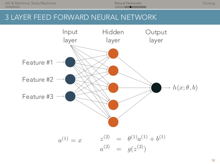
Above, $g$ is the activation function of each neuron. To make things simple all neurons have the same activation function. This three layer architecture is best described by two matrices $\theta^{(1)}$ and $\theta^{(2)}$ of parameters. These are the parameters that the model learns, as described in the previous section. $\theta^{(1)}$ and $\theta^{(2)}$ are needed to compute the output of each layer $(1)$ and $(2)$, and ultimately $h(x^i, \theta)$. Conclusion, $h$ is thus computed as a sequence of matrix-vector multiplications. This sequence of operations, called feed forward can be seen in the code snippet below:
class NeuralNet(Model):
  ...
  def _feed_forward(self, features: np.ndarray) -> np.ndarray:
      a = add_bias(features)
      for layerIndex, theta in zip(range(self.n_layers), self.thetas):
          z = np.dot(a, theta.transpose())
          sigmoid = Activation.sigmoid(z)
          if layerIndex < self.n_layers - 2:
              a = add_bias(sigmoid)
          else:
              a = sigmoid
      return a
- Point taken, then, that the most convenient way to represent the parameters of a FFNN internally – for
predictionto be efficient – is alist of matrices.
What datastructure for $\theta$ ?
At this point we agree there are two representations possible for $theta$: a vector representation and a list of matrices representation. Which one is best?
Let’s recall what the reshape function does, docs here:
>>> import numpy as np
>>> a = np.arange(4)
>>> a
array([0, 1, 2, 3])
>>> b = a.reshape((2,2))
>>> b
array([[0, 1],
       [2, 3]])
What happens now when one modifies a?
>>> a[1] = 10
>>> a
array([ 0, 10,  2,  3])
>>> b
array([[ 0, 10],
       [ 2,  3]])
Yes! b is in fact a reference, it is pointing to the same values as a. That is, the actual elements of a and b are the same. Let’s confirm this:
>>> b[1,0] = 20
>>> a
array([ 0, 10, 20,  3])
>>> b
array([[ 0, 10],
       [20,  3]])
It is therefore possible to work with one parameter set, and have two representations in our neural network implementation. That comes really handy for this specific problem! One can then define theta as a vector of parameters. This will be used for the optimization. And another representation thetas as a list f matrices, this time used for the feed forward and back propagations. Below the two code snippets which do this:
class NeuralNet(Model):
    def __init__(self, layers: List):
      ...
      self.layers = layers
      self.n_layers = len(layers)
      self.n_parameters = sum([next_layer * (layer + 1) for layer, next_layer in zip(layers[:-1], layers[1:])])
      self.theta = np.empty(self.n_parameters)
      self.thetas = []
      self._decompose(self.theta, self.thetas)
class NeuralNet(Model):
  ...
  def _decompose(self, theta: np.ndarray, thetas: List) -> List[np.ndarray]:
    idx = 0
    for l, next_l in zip(self.layers[:-1], self.layers[1:]):
        n_params = next_l * (l + 1)
        thetas.append(theta[idx:idx+n_params].reshape((next_l, l + 1)))
        idx += n_params
Conclusion
In order to train Feed Forward Neural Networks, one needs two representations of the same parameter set $\theta$:
- In the
learningphase, when performing the minimization of the loss function, $\theta$ is best represented as avector. - In the
predictionphase however, it is easier to represent $\theta$ as alist of matrices, for both the feedforward pass and the backpropagation.
In Python, numpy arrays come very handy so solve this duality. One can have two representations of the same object, either as vector or list of matrices. This is cleverly done with the reshape function.
For the complete implementation of this Feed Forward Neural Net, please visit the repo here.